Code
chart_hard_hit(batting)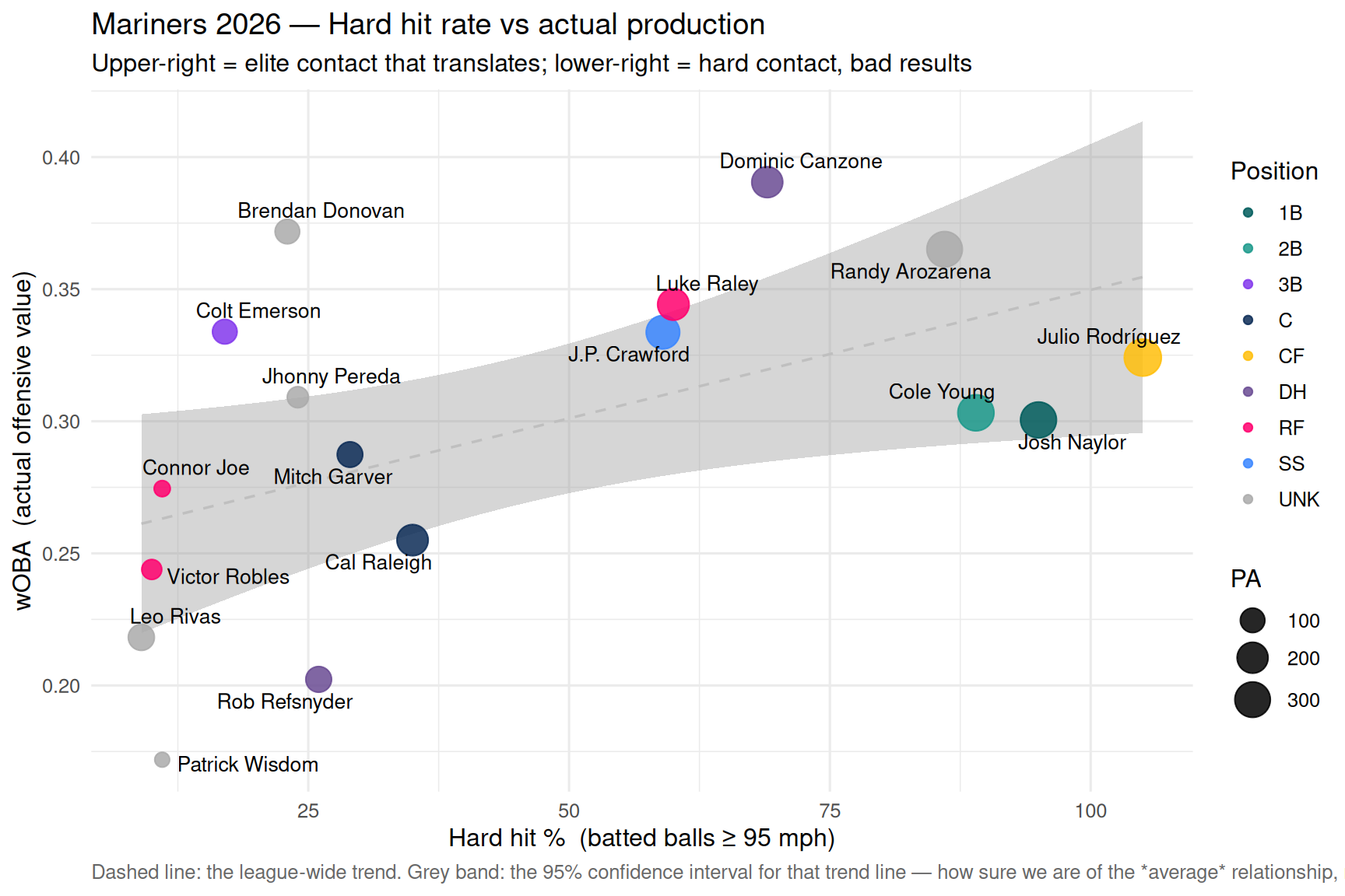
Stats, refreshed the morning after every game
Last refreshed: June 22, 2026 at 9:40 PM PDT
This site treats a baseball season like a bioinformatics experiment: players are samples, their offensive stats are features, and we look for the hitters and pitchers behaving differently from the rest. The numbers come from FanGraphs and the MLB Stats API and are re-rendered automatically the morning after each Mariners game.
Read the full differential analysis →
Hard contact vs results. Does hitting the ball hard translate into production? The dashed line is the league-wide trend; the grey band is its 95% confidence interval (how sure we are of that average relationship — not a per-player normal range). Players well above the line are out-producing their contact quality (lucky or crafty); well below, under-producing (unlucky or poor launch angles).
chart_hard_hit(batting)
BABIP — luck on balls in play. League average is ~.300; sustained extremes are rare, so red bars tend to cool off and navy bars tend to warm up.
chart_babip(batting)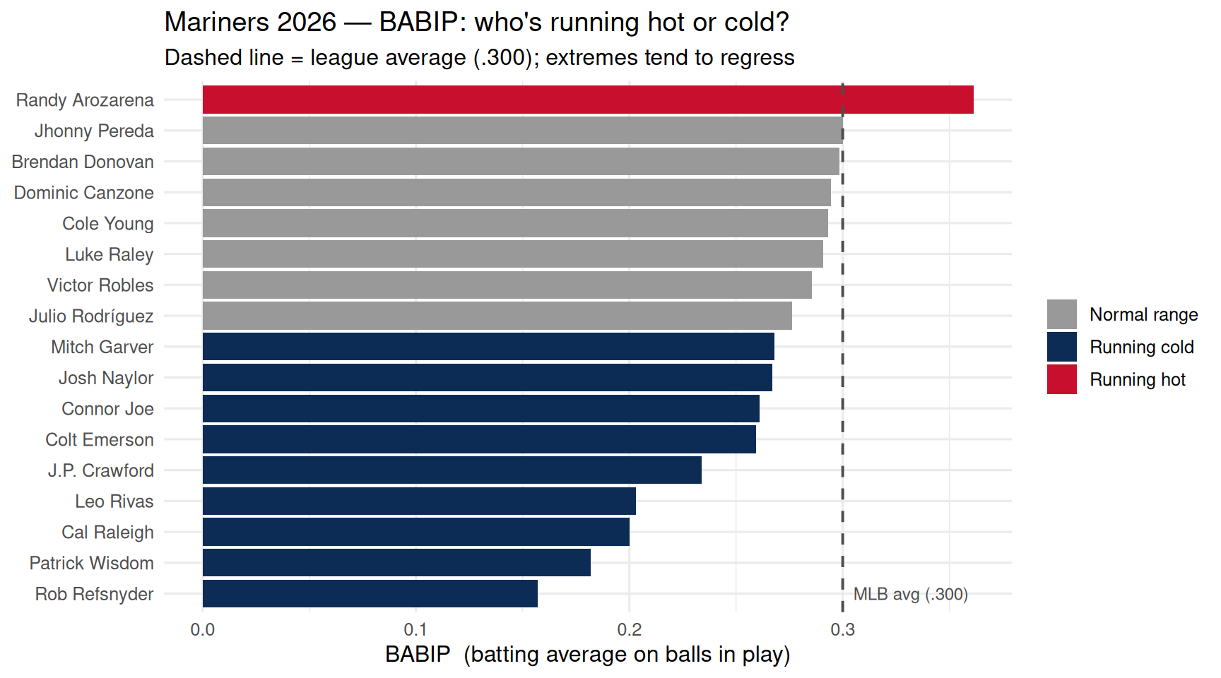
Pitching: ERA vs the peripherals. Negative bars mean a pitcher has allowed fewer runs than his strikeouts, walks, and contact quality would predict.
chart_pitching_luck(pitching)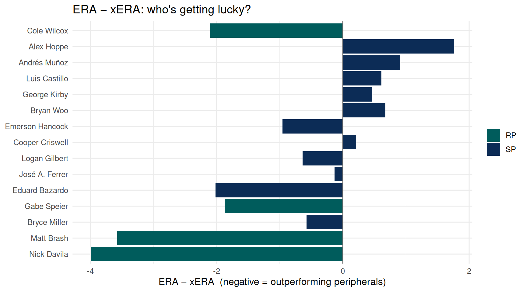
The biggest gaps between what hitters have actually produced (wOBA) and what their batted-ball quality says they should have produced (xwOBA).
glance <- batting |>
  dplyr::transmute(
    Player = player,
    Pos    = pos,
    PA     = pa,
    wOBA   = round(woba, 3),
    xwOBA  = round(xwoba, 3),
    Diff   = round(woba - xwoba, 3)
  ) |>
  dplyr::arrange(dplyr::desc(Diff))

over  <- dplyr::slice_max(glance, Diff, n = 5, with_ties = FALSE)
under <- dplyr::slice_min(glance, Diff, n = 5, with_ties = FALSE) |>
dplyr::arrange(Diff)knitr::kable(over, row.names = FALSE)
knitr::kable(under, row.names = FALSE)Running hot — over-performing
| Player | Pos | PA | wOBA | xwOBA | Diff |
|---|---|---|---|---|---|
| Colt Emerson | 3B | 101 | 0.334 | 0.228 | 0.105 |
| Brendan Donovan | UNK | 101 | 0.372 | 0.345 | 0.027 |
| Randy Arozarena | UNK | 302 | 0.365 | 0.353 | 0.012 |
| Dominic Canzone | DH | 201 | 0.390 | 0.384 | 0.006 |
| Mitch Garver | C | 112 | 0.287 | 0.295 | -0.007 |
Running cold — under-performing
| Player | Pos | PA | wOBA | xwOBA | Diff |
|---|---|---|---|---|---|
| Patrick Wisdom | UNK | 44 | 0.172 | 0.265 | -0.093 |
| Connor Joe | RF | 45 | 0.274 | 0.337 | -0.063 |
| Rob Refsnyder | DH | 115 | 0.202 | 0.257 | -0.055 |
| Cal Raleigh | C | 205 | 0.255 | 0.293 | -0.038 |
| Jhonny Pereda | UNK | 68 | 0.309 | 0.346 | -0.037 |
Pitching staff — ERA − xERA
pitching |>
  dplyr::transmute(
    Player = player,
    Role   = role,
    IP     = ip,
    ERA    = round(era, 2),
    xERA   = round(xera, 2),
    `ERA − xERA` = round(era_minus_xera, 2)
  ) |>
  dplyr::arrange(`ERA − xERA`) |>
knitr::kable(row.names = FALSE)| Player | Role | IP | ERA | xERA | ERA − xERA |
|---|---|---|---|---|---|
| Nick Davila | RP | 12.2 | 0.00 | 3.99 | -3.99 |
| Matt Brash | RP | 16.2 | 0.54 | 4.11 | -3.57 |
| Cole Wilcox | RP | 13.1 | 5.40 | 7.50 | -2.10 |
| Eduard Bazardo | SP | 34.1 | 2.10 | 4.12 | -2.02 |
| Gabe Speier | RP | 18.2 | 1.93 | 3.80 | -1.87 |
| Emerson Hancock | SP | 85.0 | 3.60 | 4.56 | -0.96 |
| Logan Gilbert | SP | 93.0 | 3.29 | 3.93 | -0.64 |
| Bryce Miller | SP | 40.0 | 1.57 | 2.15 | -0.58 |
| José A. Ferrer | SP | 32.0 | 2.81 | 2.94 | -0.13 |
| Cooper Criswell | SP | 30.2 | 3.52 | 3.31 | 0.21 |
| George Kirby | SP | 90.0 | 4.10 | 3.63 | 0.47 |
| Luis Castillo | SP | 70.2 | 5.22 | 4.61 | 0.61 |
| Bryan Woo | SP | 89.0 | 3.94 | 3.27 | 0.67 |
| Andrés Muñoz | SP | 27.1 | 5.27 | 4.36 | 0.91 |
| Alex Hoppe | SP | 22.0 | 5.32 | 3.56 | 1.76 |
How this updates: a scheduled GitHub Actions workflow checks each morning whether the Mariners finished a game the night before. If so, it re-fetches the stats, re-renders this site, and deploys it to Vercel. Off-days are skipped, and the synthetic fallback is never published.